MAP Procedure

Reference Guide > M–N Routines > MAP Procedure

MAP Procedure

Plots a map dataset.

Usage

MAP

Input Parameters

None.

Keywords

Axes—If present and nonzero, draws coordinate axes on the map plot.

note

The Axes keyword labels the points where meridians or parallels cross the border of a plot. Because of inaccuracies of the reverse projection algorithms used to accomplish this, the labeling can sometimes be omitted or be incorrect for wide area plots and certain projection methods. In general, when a smaller area is plotted, the labeling is correct.

Background—Specifies a solid background color when the Projection keyword is set to 99 (3D mapping onto sphere). If set to –1, creates a light source shaded background. The default is 0 (zero), no background.

Boundary—If specified, plots the boundary calculated by the Exact keyword. The color used is set by the Gridcolor keyword. This keyword has no effect if the Exact keyword is not set. Boundary = n specifies a boundary line thickness of n pixels; if n > 1 a more accurate line clipping algorithm is employed.

Center—(float) Array containing a longitude and latitude value that defines the center of the geographic area to be displayed. This keyword is an alternative to using the Range keyword. Use this keyword in conjunction with the Zoom keyword to specify the center of the area to zoom in on. Default: [–50.0, 0.0].

Color—(integer) Specifies the plot color for lines. Default is !P.Color. If set to –1, the colors defined in the dataset are used. This keyword can specify a scalar or an array containing a different color for each line segment or polygon. See the Discussion section for more information.

Data—(string) Specifies the name of the map dataset to plot. Datasets provided with PV‑WAVE include World Dataset II (world_db) and USGS Digital Line Graph Dataset (usgs_db). (Default: world_db)

Exact—If specified, MAP attempts to fit the map area exactly to the latitude/longitude lines specified by the Range or Center/Zoom keywords. The aspect ratio of the resulting map is also correct, and the largest map possible that fits in the window/position is produced. The Exact keyword projects points along the latitude/longitude boundary specified by the Range or Center/Zoom keywords and uses the minimum and maximum values of the projected data to establish the data coordinate system. The Exact keyword usually results in very precise map ranges, but can fail for some projections if a singularity (like one of the poles) exists within the range specified. If such a singularity exists, then the default range calculation is used. (Default: off)

File_Path—(string) Specifies the path to a file that will contain the data extracted from the selected dataset. The data is stored in a binary XDR format, and can be read in again using the Read_Path keyword.

Filled—If present and nonzero, uses the MAP_POLYFILL procedure to create a polygon-filled map rather than a line (vector) plot. Of the two map datasets supplied with PV‑WAVE, only the usgs_db dataset can be filled. To fill a state, you must set the COUNTY field to –1 (using the Select keyword). To fill multiple states, you must make separate calls to MAP.

GridColor—(integer) Specifies the line color of the grid overlay. The GridColor default is !P.Color.

GridLat—(integer) Specifies the default spacing of latitude lines, measured in degrees. (Default: 10 degrees)

GridLines—If present and nonzero, overlays a grid on the map projection.

GridLong—(integer) Specifies the default spacing of longitude lines, measured in degrees. (Default: 15 degrees)

GridStyle—(integer) Specifies the linestyle of the grid overlay, as shown in Grid Overlay Linestyles.

Table 11-1: Grid Overlay Linestyles
Index	X Windows Style	Windows Style
0	Solid	Solid
1	Dotted	Short dashes
2	Dashed	Long dashes
3	Dash dot	Long-short dashes
4	Dash-dot-dot-dot	Long-short-short dashes
5	Long dashes	Long dashes

The Windows linestyles are only available on Windows platforms and affect only the following device drivers:

WIN32—The standard windows display driver.

WMF—The Windows Metafile driver.

PM—The PixMap driver.

All other device drivers use the UNIX linestyles exclusively.

The Windows drivers listed above use the Windows linestyles by default. You may force the Windows drivers listed above to use the UNIX linestyles by setting the PV-WAVE system variable !UNIX_LINESTYLES to 1. (Default: !UNIX_LINESTYLES = 0)

The Gridstyle default is !P.Linestyle.

Image—Specifies an image (2D array) to be warped around the map projection and displayed with the map lines. If the image array is not of type byte, it will be automatically passed through the BYTSCL procedure before being plotted. The image will be warped to exactly cover the area specified using the Range keyword.

Parameters—(double) Specifies an array of up to 10 elements containing parameters to be passed to a map projection. The only built-in projection methods that use these parameters are the conic projections. The parameters currently used by the built-in projections are defined as follows:

parameter(0)—The first secant intersection. (Default: 33 degrees north)

parameter(1)—The second secant intersection. (Default: 45 degrees north)

Position—(float) The position of the map within the plot device in normal coordinates. For example, Position = [.1,.1,.9,.9] leaves a border around the map 1/10 the screen size. The Position default is the value of !P.Position.

Projection—(integer) Specifies the type of projection (see the Discussion section for a table of projection types). (Default: 1, equidistant cylindrical)

Radius—(float) Specifies a 2D array of the same size as the one specified by the Image keyword. The radius array will be used to modify the shape of the sphere used with Projection=99. The size of the array should be normalized to values between zero and one for best results. This keyword can be used to create a sphere with geographical relief displayed. The map data may not line up exactly with the radius of the sphere.

Range—(float) [lon1, lat1, lon2, lat2] Array of four points representing the lower-left and upper-right longitude/latitude coordinates of the region to be displayed. Used to specify the exact geographical area to display. An alternative method of area selection is to use the Center and Zoom keywords.

Read_Path—(string) Used to specify the name of a file created with the File_Path keyword. The data contained in this file is projected and plotted. Specifying this keyword causes the Data, Select, and Resolution keywords to be ignored.

Resolution—(integer) The effect of this keyword depends on which map dataset is used, the default world_db dataset or the usgs_db dataset:

(If the world_db dataset is used, the default) Provides a way to speed up the projection and plotting of large datasets. Specifies the number of data points to skip when a dataset is plotted. For example, Res=30 means skip every 30th point in the dataset. Specifying a larger value for this keyword results in faster plotting times, but poorer image quality. Specifying smaller values results in slower plotting times, but gives improved image quality. The default value is chosen based on the range of the map and is optimized for the 300,000 points in the world_db dataset. A reasonable range of values for the world_db dataset is between one and 30.

(If Data=’USGS_DB’) Resolution is not a measure of how many points to skip when sampling, as is done with the default map dataset, but a measure of the minimum distance (in latitude/longitude) between points. Resolution values should range between 0.01 and 0.2 for good results. The sampling is not used for county boundaries, or for Hawaii and Alaska. The code to sample the data is slow, so should be used with the File_Path keyword of the MAP procedure to save the sampled map, which can be later displayed with the Read keyword of the MAP procedure. (Default: off)

Save—If present and nonzero, saves the 3D scaling parameters in !P.T to allow overplotting of other data. This keyword is only used when the Projection keyword is set to 99 (3D mapping onto a sphere).

Select—(unnamed structure) Specifies a subset of the dataset to plot. See the Discussion for more information on this keyword.

Stretch—If present and non-zero causes the plot area to be scaled to the actual range of data points extracted from the dataset. This stretches any subset of data to occupy the entire plot area. (See the Discussion section for more information.)

User—(string) Specifies the name of a user-defined projection procedure. If this keyword is used, then the Projection keyword is automatically set to –1.

Zoom—(float) Specifies a factor by which the display is magnified or reduced around a center point specified with the Center keyword. For example, a factor 2 magnifies the region surrounding the center point by two times. The default value is 1.0.

Standard Plotting Keywords

The following standard plotting keywords are used with MAP. See Graphics and Plotting Keywords for more information.

Linestyle	Line_Fill	Spacing	Threshold
Pattern	NoData	Orientation
Fill_Pattern	NoErase	Thick

Discussion

When you use the Center and Zoom keywords to specify map bounds, if the center latitude is either –90 or 90, it is assumed that you want a polar view, and the longitude range is forced to –180 to 180. In other words the Zoom parameter will only affect the range of latitudes about the pole and not the longitude range.

Map Projections

You can produce the map projections shown in Map Projections with the MAP procedure. To specify a projection, set the Projection keyword to the corresponding map projection index number.

Table 11-2: Map Projections
Index	Projection	Index	Projection
1	Equidistant Cylindrical	11	Oblique Azimuthal Equidistant Oblique
2	Lambert Conformal Conic	12	Polar Azimuthal Equidistant Oblique
3	Cylindrical Mercator	13	Polar Azimuthal Equal-Area
4	Sinusoidal	14	Oblique Azimuthal Equal-Area
5	Albers Equal-Area Conic	15	Transverse Mercator
6	Polyconic	16	Mollweide (Ellipsoid)
7	Polar Stereographic	99	Satellite (3D mapping onto a sphere)
8	Oblique Stereographic*	–1	User-defined projection (automatically set if the User keyword is supplied)
9	Oblique Orthographical*	0	No projection
10	Polar Orthographical
* Oblique projections can be used at the poles as follows: map,range=[-180,0,180,180],/exact,proj=9,boun=2,sel={,group:['cil']},res=0 map,range=[-180,-180,180,0],/exact,proj=9,boun=2,sel={,group:['cil']},res=0

Map Stretch

By default the data area used by MAP is a rectangle scaled to the values specified in the Range or the Center and Zoom keywords (converted to radians). This usually gives good results, but there is sometimes a border around the map due to the particular mapping projection algorithm being used. Specifying Stretch resizes the plot area to the actual range of the projected data extracted and causes the map to always fill the entire plot area. This can change the aspect ratio of the map (height to width ratio), but is useful when a map needs to exactly cover a specified area on the device, such as when a cylindrically projected map is displayed over an image which was displayed using the TV command.

Subsetting Datasets

The Select keyword is used to specify subset criteria for the map dataset. Datasets included with PV‑WAVE include World Databank II (world_db) and USGS Digital Line Graph (usgs_db) datasets.

note	The World Databank II dataset is a subset of a public domain dataset provided by the U.S. Department of Commerce, merged with updated country data from the National Imagery and Mapping Agency (NIMA).

You can subset the world_db dataset by passing an unnamed structure via the Select keyword. Table 11-3: Example Structure Fields on page 767 lists the possible fields and tags of this structure.

Table 11-3: Example Structure Fields
Fields	Tags
GROUP	CIL—Coastlines, islands, lakes
	BDY—International boundaries
	PBY—Primary/First Order (internal) boundaries such as, U.S. States).
	RIV—Major rivers
AREA	As of Version 7.0, this field is obsolete. If AREA is specified, it is ignored.

note	If the field is set to a null string, all tags are plotted.

You can subset the usgs_db dataset by passing an unnamed structure via the Select keyword. The following lists the possible fields and tags of this structure:

STATE—One or more FIPS codes for the states to plot (two-letter state abbreviations can also be used—AL, AK, AZ, AR, CA, etc.).

COUNTY—One or more FIPS codes for the counties to plot. (–1 draws all counties; 0 draws no counties).

For example:

; World Databank II data is subsetted to plot coastlines,

; islands, and lakes in Asia.

MAP, Select={, GROUP:['CIL'], AREA:'ASIA'}

; Plot USGS Digital Line Graph data of Pennsylvania.

MAP, Data='usgs_db', Range=[-81,39,-75,43], /Gridlines, $
Gridstyle=2, Gridlat=1, Gridlong=5, $
Select={,STATE:'PA',COUNTY:-1}

note

If COUNTY is anything but 0, only the first state specified can be plotted. To plot multiple states/counties, you must make separate calls to MAP.

This USGS data is from the USGS 1:2,000,000 Scale Digital Line Graph CD. Note that some errors exist in the original data. For instance, when filling counties along coastlines, the filling will be inexact because the original polygon data for each county did not include the coastline portion.

Map Colors

The colors used when the Color keyword is set to –1 are colors that are assigned within the map dataset. If you want to use the dataset colors, you may have to use a custom color palette or the TEK_COLOR procedure. The colors returned by the datasets that are provided with PV‑WAVE are as follows:

Color assignments in the WORLD_DB dataset:

Coastlines/Islands/Lakes—Color = 1

Rivers—Color = 2

International Boundaries—Color = 3

Primary Boundaries—Color = 4

Color assignments in the USGS_DB dataset:

For State plots (COUNTY tag field = 0): Color = State FIPS code

For County plots: Color = County FIPS code

The colors are modulus the number of display colors if the FIPS codes exceed !D.N_Colors.

Examples

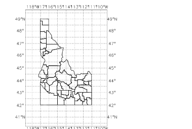
This example produces a filled map of Idaho as shown in Figure 11-1: Map of Idaho on page 769. Keywords are used to set the map range, select the map dataset, subset the dataset, add gridlines and axes.

TEK_COLOR

!P.background = WoColorConvert(1)

!P.position = [0.3, 0.1, 0.7, 0.9]

MAP, Range=[-118.0, 40.5, -110.0, 50.0], Data='usgs_db', $

   Select={, state:'ID', county:-1}, Thick=2, /Axes, $

   /Gridlines, GridColor=WoColorConvert(0), Gridstyle=1, $

   Gridlong=1, Gridlat=0.5, Color=WoColorConvert(9)

Figure 11-1: Map of Idaho

File_Path and Read_Path Keywords

The File_Path and Read_Path keywords allow you to create a data subset which can be read and reused without re-reading and re-subsetting the entire dataset.

These keywords can greatly increase the performance of your application. To use these keywords, specify a file pathname when you select a subset of the data, as in this example:

MAP, DATA='world_db', RANGE=[-150, 30, 30, 70], $
SELECT={, GROUP:'cil'}, RESOLUTION=20, FILE_PATH='mymap.dat'

You can now plot this map or subareas of this map without reading the entire world_db dataset, as in this example:

MAP, Range=[-150, 30, 30, 70], Projection = 4, $
Read_Path = 'mymap.dat'