VELOVECT Procedure

Reference Guide > U–V Routines > VELOVECT Procedure

VELOVECT Procedure

Standard Library procedure that draws a two-dimensional velocity field plot, with each arrow indicating the magnitude and direction of the field.

Usage

VELOVECT, u, v[, x, y]

Input Parameters

u—The x component of the two-dimensional field. This parameter must be a two-dimensional array.

v—The y component of the two-dimensional field. This parameter must be a two-dimensional array of the same size as u.

x—(optional) The abscissa values. This parameter must be a vector whose size equals the first dimension of u and v.

y—(optional) The ordinate values. This parameter must be a vector whose size equals the second dimension of u and v.

Keywords

Dots—If present and nonzero, places a dot at the position of the missing data. Otherwise, nothing is drawn for missing points. Dots is only valid if the Missing keyword is also specified.

Length—A length factor. The default value is 1.0, which makes the longest (u, v) vector have a length equal to the length of a single cell.

Missing—A two-dimensional array with the same size as the u and v arrays. It is used to specify that specific points have missing data.

If the magnitude of the vector at (i, j) is less than the corresponding value in Missing, then the data is considered to be valid. Otherwise, the data is considered to be missing.

Thus, one way to set up a Missing array is to initialize all elements to some large value:

missing_array = FLTARR(n, m) + 1.0E30

Then, if point (i, j) is a missing point, set the corresponding element to a negative value:

missing_array(i, j) = -missing_array(i, j)

Discussion

VELOVECT draws a two-dimensional velocity field plot. The arrows indicate the magnitude and the direction of the field.

If missing values are present, you can use the Missing keyword to specify that they be ignored during the plotting, or the Dots keyword to specify that they be marked with a dot.

The system variables ![XY].Title and !P.Title may be used to title the axes and the main plot.

Examples

These examples create the figures shown in Figure 18-5: Velocity Field with Default Values on page 1407, Figure 18-6: Velocity Field with Modified Arrows on page 1407, and Figure 18-7: Velocity Field with Missing Data on page 1408.

; Create the arrays.

u = FLTARR(21, 21)

v = FLTARR(21, 21)

; Type .RUN, the WAVE prompt changes to a dash (–) to indicate

; that you may enter a complete program unit.

.RUN

; This procedure stuffs values into arrays; the last END exits the

; programming mode, compiles and executes the procedure, and

; then returns you to the WAVE prompt.

   FOR j=0L, 20 DO BEGIN

      FOR i=0L, 20 DO BEGIN

         x=0.05 * FLOAT(i)

         z=0.05 * FLOAT(j)

         u(i, j) = -SIN(!Pi*x) * COS(!Pi*z)

         v(i, j) = COS(!Pi*x) * SIN(!Pi*z)

      ENDFOR

   ENDFOR

END

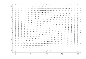
; Display the velocity field with default values.

VELOVECT, u, v

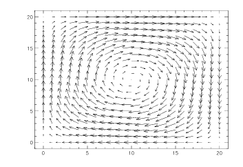
; Display the velocity field using arrows twice the length of a

; single cell.

VELOVECT, u, v, Length=2

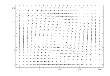
missing = FLTARR(21, 21) + 1.e30

missing(4:6, 7:9) = -1.e30

missing(15:17, 16:19) = -1.e30

; Display the velocity field that contains missing data.

VELOVECT, u, v, Missing=missing, /Dots

Figure 18-5: Velocity Field with Default Values

Figure 18-6: Velocity Field with Modified Arrows

Figure 18-7: Velocity Field with Missing Data