Produces an evenly sampled grid from scattered data.

xvec—An array of floating-point values containing the x coordinates of the input data.

yvec—An array of floating-point values containing the y coordinates of the input data.

zvec—An array of floating-point values containing the z coordinates of the input data.

Bounding_Poly—A (2,*) floating-point array specifying the vertices of a polygon describing the outer boundary of the resulting grid. The first and last points of the polygon must be identical.

Dist_Avg—(float) Specifies the distance over which to average input points before using them to compute the grid nodes. In general, the value of Dist_Avg is a fraction of the grid spacing (Xspacing/Yspacing keywords), but you can minimize the number of points processed by increasing the value of Dist_Avg. (Default: MIN([xspacing, yspacing])/2)

Interp_Dist—(float) Specifies the maximum distance, in the same units as xvec and yvec, to interpolate from each point. (Default: MAX([xmax-xmin, ymax-ymin])*radius/200.0) Where radius is expressed as a percentage. See the Radius keyword.

Method—The Method keyword is a string value used to specify how primary gridding estimates at grid nodes are performed. Primary estimates are discussed in the section "Primary Estimates of Z Values". The arguments for the Method keyword are: Direct, Scatter, Cluster, and Weighted. These arguments are discussed in the section "Method Keyword Arguments".

Neighbors—(integer) Specifies the number of octants required to have neighbors before calculation of a node is attempted. For extrapolation, use Neighbors=3. (Default: 5)

Nodestroy—If nonzero, preserves the surface information. By default, the memory allocated for the surface information is freed.

Nomessage—If nonzero, messages that are output while the GTGRID function is running are not displayed. By default, messages are displayed.

Nsmooth—(integer) Specifies the number of smoothing passes made on the data. The default is 20. For more information on smoothing, see "Smoothing".

Nulval—(float) Specifies the numeric value used by the gridder for null or missing grid nodes in the resulting output grid. The default value is determined by inspecting the zvec array and computing:

Nulval = min(ZVEC) - (max(ZVEC) - min(ZVEC))

This is designed to ensure a reasonable presentation of the output grid by PV-WAVE commands such as SURFACE.

Nx—(integer or long) Specifies the first dimension of the result array. If Nx is not specified, but Ny is specified, then Nx is set equal to Ny. (Default: 20)

Ny—(integer or long) Specifies the second dimension of the result array. If Ny is not specified, but Nx is specified, then Ny is set equal to Nx. (Default: 20)

Radius—(float) Specifies distance, expressed as a percentage of the greater of (xmax – xmin) or (ymax – ymin), over which interpolation will be performed. This keyword is used by all the gridding methods except for Direct. (Default: 50 percent)

One interpretation of this parameter is to consider it as the distance at which the covariance function goes to zero. Points that are farther away from each other than this are essentially independent.

A larger value of Radius is occasionally required when the input points are distributed such that large gaps exist in the coverage. A larger value of Radius will slow processing down.

A smaller value of Radius is useful for speeding things up, and can be used to generate surfaces that have holes wherever there is no coverage.

Surf_id—(long) Returns a value used to reference surface information internal to the GTGRID libraries. This value is used as input to other PV‑WAVE GTGRID functions and procedures. Use the Nodestroy keyword with the Surf_id keyword to preserve surface information in memory for future access.

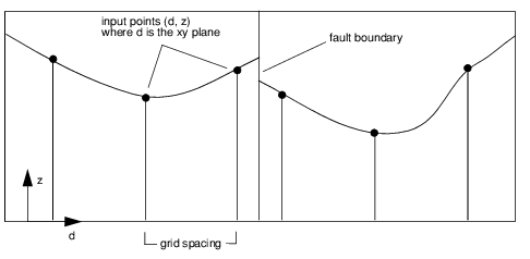
Xfaults—A 1D array of floating-point values used to define faults relative to the xvec parameter. The values for Xfaults must be defined within the same coordinate system as xvec. There is no default for this keyword. To provide multiple faults, use the value 0.0 as the separator between each fault. If Xfaults is present, but Yfaults is not provided, an error message is produced and GTGRID returns the scalar 0.0 as the results. Interpolated Curve with a Fault represents an interpolated curve with a fault.

Xmax—(float) Defines the maximum x grid boundary in data coordinates. The default is the maximum value found in xvec.

Xmin—(float) Defines the minimum x grid boundary in data coordinates. The default is the minimum value found in xvec.

Xorg—(float) Specifies the x-coordinate of the origin of the generated grid. (Default: Xmin)

Xspacing—(float) Specifies the spacing between consecutive nodes in the x direction. (Default: (xmax-xmin)/(nx-1))

Yfaults—A 1D array of floating-point values used to define faults relative to the yvec parameter. The values for Yfaults must be defined within the same coordinate system as yvec. There is no default for this keyword. To provide multiple faults, use the value 0.0 as the separator between each fault. If Yfaults is present, but Xfaults is not provided, an error message is produced and GTGRID returns the scalar 0.0 as the results.

Ymax—(float) Defines the maximum y grid boundary in data coordinates. The default value is the maximum value found in yvec.

Ymin—(float) Defines the minimum y grid boundary in data coordinates. The default is the minimum value found in yvec.

Yorg—(float) Specifies the y-coordinate of the origin of the generated grid. (Default: Ymin)

Yspacing—(float) Specifies the spacing between consecutive nodes in the y direction. (Default: (ymax-ymin)/(ny-1))

Zresolution—(float) Specifies the minimum meaningful difference in z values during gridding. (Default: the value of the Nulval keyword)

The range covered by the grid is determined from the values of the Nx, Ny, Xorg, Yorg, Xspacing, and Yspacing keywords as follows:

If you generate many large grids, without destroying the internal GT surface storage, you may run out of memory. Therefore, it is wise to let GTGRID destroy your surfaces if you are calling it successively while adjusting your gridding parameters.

Once you are satisfied with the gridding parameters, use the /Nodestroy keyword; the surface ID of that generated surface can then be used by other PV‑WAVE GTGRID 3.0 functions.

When you are finished working with a surface, you can destroy it using the GTDESTROYSURF procedure. If you do not know the ID of your surface, you can use the GTGETSURFS function to obtain a list of the active GT surfaces.

Method Comparisons summarizes the advantages and disadvantages of each method and the types of data best suited to each method. The methods are described in detail in following sections.

For an example of a GTGRID call that uses the Method keyword, see examples 5 and 7 in Examples.

The Direct method provides an approximation for generating a minimum curvature solution. This method can only be used on data that contains less than 100,000 points. Use of this approach is recommended wherever it is possible. It is the fastest gridding method for small data sets, and also tends to produce the most visually pleasing results.

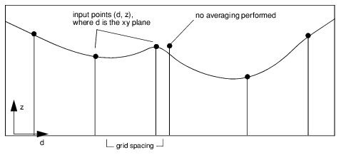
All nodes are calculated regardless of the input point distribution. The resulting surface as represented by the z values at each node in the grid is the exact solution to a set of equations that approximates the relationships among a thin metal plate, a set of desired displacements at the random input points, and the forces applied at each point.

By solving this system of equations the necessary values of the force are determined at each point. These values are then used to compute the plate displacement at every grid node. If no averaging is performed, this solution provides a surface that passes through every point specified and has the least amount of curvature possible, as shown in Interpolated Curve, without Averaging.

The Scatter method uses the Radial Search for Scattered Points algorithm. This is the default method for GTGRID.

The radial search uses randomly positioned input points to compute grid nodes in the “immediate vicinity” of each input point.

The radial search technique relies on localized fits of a plane to the selected subsets of the input points. Using each input point as an origin, a subset of the surrounding points is formed by selecting the nearest two points in each octant about the origin. Each point is then weighted according to its displacement from the origin. The plane is also constrained to pass through the point selected as the origin.

If a successful fit is accomplished, the grid nodes about the point selected as an origin are then assigned z values.

Only grid nodes that are interior to the convex hull of the input data point distribution will be assigned a z value. (The convex hull is a boundary that encompasses all the data points. For example, if each data point were a nail in a board, the convex hull could be represented by a rubber band stretched around all the nails.) This is done to minimize edge effects that are inherent to this approach.

This process repeats using every input point as an origin. GTGRID attempts to assign all unassigned grid nodes during secondary gridding. Note that some grid nodes are computed more than once if the input point distribution is such that more than one point is contained within a grid cell.

The Cluster method uses the Radial Search for Clustered or Linear Data algorithm. The Cluster Method differs from the Scatter Method in that additional effort is employed during calculation of grid nodes near input points to minimize the extrapolation of excessive gradients due to noise or points that are very close together.

Therefore, it is recommended that this method be used especially if noisy or clustered data is being processed.

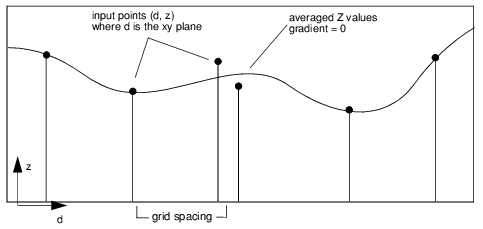
This method uses the Weighted algorithm. This is a relatively fast method of mapping points onto a specified grid without any attempt at interpolation or gradient estimation.

Use this method if you want to input a set of values which were computed on a grid by a modeling program or if an abundance of data is available relative to the grid size desired. Each grid node is a weighted combination of the data points surrounding it within adjacent cells. Secondary gridding is then employed to fill unassigned grid nodes. If the input distribution is fairly uniform, this method is much faster than the others. Interpolated Curved via Weighted Method shows the curve fit produced with this method.