Drawing a Surface
The SURFACE procedure draws “wire mesh” representations of functions of X and Y, just as CONTOUR draws their contours. Parameters to SURFACE are similar to CONTOUR. SURFACE accepts a two-dimensional array of Z (elevation) values, and optionally x and y parameters indicating the location of each Z element.
SURFACE projects the three-dimensional array of points into two dimensions after rotating about the Z and then the X axes. Each point is connected to its neighbors by lines. Hidden lines are suppressed. The rotation about the X and Z axes can be specified with keywords, or a complete three-dimensional transformation matrix can be stored in the field !P.T, for use by SURFACE. Details concerning the mechanics of 3D projection and rotation are covered in the next sections.
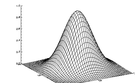
The following code illustrates the most basic call to SURFACE. It produces a two-dimensional Gaussian function and then calls SURFACE to produce
Gaussian Surface Plot.
; Create 40-by-40 array, shift origin to center of array.
z = SHIFT(DIST(40), 20, 20)
; Form Gaussian with 1/e width of 10, and call SURFACE to display.
SURFACE, EXP(-(z/10)^2)
In the previous example, the DIST function creates an (n, n) array. DIST is a useful function for creating data, and is described in detail in the PV‑WAVE Reference.
Controlling Surface Features with Keywords
The following keywords are unique to, or have particular relevance to, the
SURFACE procedure. For a complete list of the SURFACE keywords, see the description of SURFACE in the PV‑WAVE Reference.
Ax | Horizontal | Skirt |
Az | Lower_Only | Upper_Only |
Bottom | Save | ZAxis |
For a detailed description of these keywords, see Chapter 21: Graphics and Plotting Keywords of the PV‑WAVE Reference.
Example of Drawing a Surface
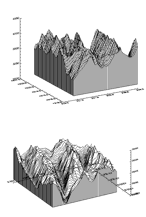
Maroon Bells Surface Plots illustrates the application of the SURFACE procedure to the Maroon Bells data discussed earlier in this chapter (see
"Drawing Contour Plots with CONTOUR").
The first illustration was produced by the following statements:
c = REBIN(a > 2650, 350/5, 460/5) SURFACE, c, x, y, SKIRT=2650
The first statement rebins the original data into a 70-by-92 array, as discussed in
"Contouring Example", while setting all missing data values (which are 0) to 2650, the lowest elevation we wish to show. As with CONTOUR, there can be too many data values, obscuring the surface with too much detail, and requiring more computation and drawing time.
The second illustration shows the Maroon Peaks area looking from the back row to the front row (north to the south), AZ = 210, and from a slightly steeper azimuth AX = 45. Also, only the horizontal lines are drawn because the Horizontal keyword assignment is present in the call:
SURFACE, c, x, y, SKIRT=2650, /Hor, AZ = 210, AX = 45
Because the axes were rotated 210 degrees about the original Z axis, the annotation is reversed and the X axis is behind and obscured by the surface. This undesirable effect can be eliminated by reversing the data array c about its Y axis. Also the y vector of element locations must be reversed, and the YRange keyword used to reverse the Y axis ordering.
; Perform as previously, but reverse data rather than axes.
SURFACE, reverse(c ,2), x, reverse(y), Skirt = 2650, /Hor, $
AX = 45, YRange = [Max(y), Min(y)]
Version 2017.1
Copyright © 2019, Rogue Wave Software, Inc. All Rights Reserved.