Drawing Shaded Surfaces

The SHADE_SURF procedure creates a shaded representation of a surface made from regularly gridded elevation data. The shading information may be supplied as a parameter or computed using a light source model. Displays are easily constructed depicting the surface elevation of a variable shaded as a function of itself or another variable. This procedure is similar to the SURFACE routine, but it renders the visible surface as a shaded image rather than a mesh.

Parameters are identical to those of the SURFACE procedure, described in the section "Drawing a Surface", with the addition of two optional keyword parameters:

Shades—Specifies an array of the same dimensions as the Z parameter, which contains the shading color indices. This array should be scaled into the range of color indices, normally 0 to 255.

Image—Specifies the name of a variable into which the image created by SHADE_SURF is placed. Normally, the image is displayed on the currently selected graphics device and then discarded.

The shading applied to each polygon, defined by its four surrounding elevations, may be either constant over the entire cell, or interpolated. Constant shading is faster because only one shading value needs to be computed for the entire polygon. Interpolated shading gives smoother, usually more pleasing, results. The Gouraud method of interpolation is used: the shade values are computed at each elevation point, coinciding with each polygon vertex; then the shading is interpolated along each edge; and finally between edges along each vertical scan line.

Light source shading is computed using a combination of depth cueing, ambient light, and diffuse reflection, adapted from Chapter 16 of Fundamentals of Computer Graphics, Foley and Van Dam:

Ia is the term due to ambient light. All visible objects have at least this intensity, which is approximately 20% of the maximum intensity.

Ip(L · N) is the term due to diffuse reflection. The reflected light is proportional to the cosine of the angle between the surface normal vector N, and the vector pointing to the light source L. Ip is approximately 0.9.

d is the term for depth cueing, causing surfaces further away from the observer to appear dimmer. d = (z+2)/3, where z is the normalized depth, ranging from zero for the most distant point, to one for the closest.

Parameters affecting the method of shading interpolation, light source direction, and rejection of hidden faces are set with the SET_SHADING procedure, described in the PV‑WAVE Reference. Defaults are: Gouraud interpolation, light source direction is [0, 0, 1], and rejection of hidden faces enabled.

See the description of SET_SHADING in PV‑WAVE Reference for a more complete description of the parameters. Note that the Reject keyword has no effect on the output of SHADE_SURF—it is used only with solids.

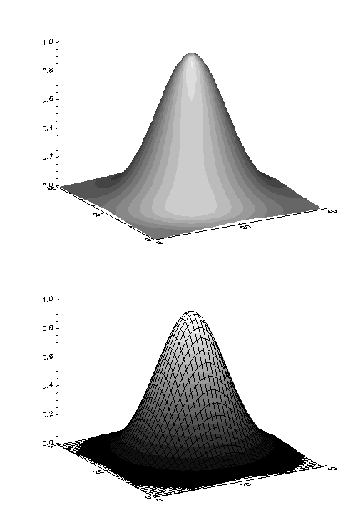
The left side of Shaded 2D Gaussian Plots illustrates the application of SHADE_SURF, with light source shading, to the two-dimensional Gaussian, z, used to produce Figure 5-10: Gaussian Surface Plot on page 97. This figure was produced by the statement:

The first image of Shaded 2D Gaussian Plots shows the use of an array of shades, which in this case is simply the surface elevation scaled into the range of bytes. The output of SURFACE is superimposed over the shaded image with the statements:

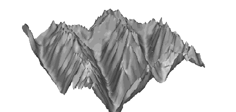
Shaded Surface of Maroon Bells shows the Maroon Bells data, also shown in the first image of Figure 5-11: Maroon Bells Surface Plots on page 100, as a light source shaded surface. It was produced by the statement:

The AX and AZ keywords specify the orientation. The axes are suppressed by the axis style keyword parameters, as in this orientation the axes are behind the surface.