Gray Level Transformations
Each pixel, or cell, in an image exhibits an intensity. By modifying the distribution of intensities it is possible to produce an image more suitable for a given application than the original. Of course, a suitable image for one application is not necessarily the best image for another application. The viewer is the ultimate judge of how well a particular method works. Evaluating image quality is a highly subjective process.
There are two ways to modify image intensities:

modify the pixels and re-write the image on the display, or
modify the color translation tables without changing the pixels.
The second method is faster because the color translation tables contain less information than the pixel memory, but it is not always practical because the original image may contain more discrete values than are representable in the display memory.
Thresholding, the Simplest Gray-level Transformation
The simplest example of a gray-level transformation is to produce a two-level mapping from all the possible intensities into black and white. If an image stored in a variable named A contains an object in which each pixel has an intensity value greater than S, a scalar, and pixels that are not part of the object have a value less than S, then the statement:
TVSCL, A GT S
will display all pixels in the object as full white and all background pixels as black.
The relational operators, EQ, NE, GE, GT, LE and LT, produce a value of 1 if the relation is true and 0 if the relation is false. When applied to images, the relation is applied to each pixel and an image of 1’s and 0’s results.
For example, the expression A GT S is an image with a value of 1 in each element where the corresponding element of A is greater than S; otherwise the element is set to 0. The TVSCL procedure then scales the image of 1’s and 0’s into 255’s and 0’s.
Of course, the opposite effect is obtained by the statement:
TVSCL, A LE S
All pixels whose value is greater than S but less than T are displayed as white with the following statement:
TVSCL, (A GT S) AND (A LT T)
Thresholding using Color Table Modification
If the original image scales into the range of integers representable in the display memory, the thresholding operators in the previous section may be implemented more efficiently by changing the color translation tables. For example, if a 256-element gray scale color table is appropriate, elements less than S become white with the following statements:
; Elements less than S are 255, others are 0.
T = 255 * (INDGEN(256) LT S)
; Load the color table from T.
TVLCT, T, T, T
Contrast Enhancement
An image may be contrast-enhanced so that any subrange of pixel values are scaled to fill the entire range of displayed brightnesses. For instance, if the image in variable A contains an object superimposed on a varying background, and the pixel values in the object range from a value of S to the brightest value in the entire image, the statement:
TVSCL, A > S
will use the entire range of display brightnesses to display the object.
The > operator, called the maximum operator, yields a result equal to the larger of its two operands. The expression A > S is an image in which each pixel in A less than S is set to S. S becomes the new minimum intensity. TVSCL then scales the new image from 0 to 255 before loading it into the display. Again, the image A is not changed. If, for example, the object in A has values from 2.6 to 9.4, the statement:
TVSCL, A > 2.6 < 9.4
truncates the image so that 2.6 is the new minimum and 9.4 is the new maximum before scaling and display. Pixels with intensities of 9.4 or larger will be displayed at full brightness, while those with intensities of 2.6 or less are converted to minimum brightness.
Using BYTSCL to Enhance Contrast
The BYTSCL function can be used to enhance the contrast of images in a more efficient manner than the examples above. The result of this function is a byte image made by scaling the input image as follows:
Rx,y = T (Ix,y – Min) / (Max – Min)
where Ix,y is the intensity value at image location (x, y). The value of T may be specified using the Top keyword parameter. Its default value is 255. If BYTSCL is called with only one parameter, the maximum and minimum values are obtained by scanning the image parameter. You may directly specify the minimum and maximum values with keyword parameters. For example, the statement:
TV, BYTSCL(A, MIN = 2.6, MAX = 9.4)
has the same effect as the TVSCL statement in the previous section, stretching the contrast of pixels ranging from 2.6 to 9.4, but this statement is considerably quicker. Using BYTSCL is more efficient because the range truncation and scaling are performed in one pass, rather than in the four required by the TVSCL statement.
Modifying Color Tables to Enhance Contrast
If the image contains pixels in the range of 0 to 255, as in the case of an 8-bit display, or it can be transformed to 256 or fewer values, it is faster to modify the display color lookup tables rather than transforming the image in the computer and then loading the display. The STRETCH procedure allows any range of values between 0 and 255 to be linearly expanded to fill the display range.
For more information about stretching color tables, see
"Stretching the Color Table", or refer to the STRETCH procedure in the PV‑WAVE
Reference.
Histogram Equalization
In many images, most pixels reside in a few small subranges of the possible values. By spreading the distribution so that each range of pixel values contains an approximately equal number of members, the information content of the display is maximized.
To equalize the histogram of display values, the count-intensity histogram of the image is required. This is a vector in which the ith element contains the number of pixels with an intensity equal to the minimum pixel value of the image plus i. The vector is of longword type and has one more element than the difference between the maximum and minimum values in the image. (This assumes a binsize of 1 and an image that is not byte type.) The sum of all elements in the vector is equal to the number of pixels in the image.
The HISTOGRAM function directly returns the count-intensity histogram. For example, to define a new variable H that contains the count-intensity histogram of the image A, type:
H = HISTOGRAM(A)
Optional keyword parameters may be included to specify the range and binsize, determine the minimum value of the image, etc.
From the count-intensity histogram, the cumulative distribution function is computed with the statements:
P = H
FOR i = 1, N_ELEMENTS(P)-1 DO P(i)= P(i) + P(i-1)
Pi now contains the number of pixels in the original image with intensities less than or equal to i:
Pi increases monotonically from the minimum value of the image to the number of pixels in the image.
By simply normalizing P so that its maximum element has a value of 255 and its minimum element has a value of 0, the gray level transformation necessary to display the image with histogram equalization is obtained:
P = BYTSCL(P)
The statement:
TVLCT, P, P, P
loads the three display color translation tables with the transformed function. The result is a black and white histogram- equalized display.
The HIST_EQUAL_CT procedure loads the color tables with a histogram equalized distribution, as described above. If called with no parameters, this procedure allows the user to mark a rectangular region of the display with the mouse, which is then used to form the distribution. It can also be called with an image as its parameter, in which case it uses the pixel distribution of the entire image.
Example of Histogram Equalization
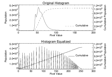
The top plot of
Figure 6-1: Histogram of Original and Histogram-Equalized Image on page 137 shows the count-intensity histogram of an original aerial image of the New York city area. The dashed line is the cumulative integral of this function, showing the number of pixels in the image with values less than or equal to each pixel value.
It is apparent that pixel intensities range from approximately 40 to 140, implying that only 40% of the usable brightness range of display is used.
The bottom plot shows the pixel distribution histogram of the histogram-equalized image. Note that the histogram is spread over a much larger range and that the shape is somewhat flattened. Not all the values in this histogram are equal. This is due to the discrete bin size of the histogram and because there are unpopulated pixel ranges.
The cumulative integral of the histogram is nearly a straight line, from the origin to an x value of the maximum pixel value and a y value equal to the number of pixels, as it should be.
The HIST_EQUAL function performs histogram equalization using this method. The following statement uses HIST_EQUAL to transform the image A and then display the result:
TV, HIST_EQUAL(A)
As described above, the HIST_EQUAL_CT procedure is more efficient because it modifies the color tables, rather than the image. The following two statements display the image, and then load the modified color tables:
TV, A
HIST_EQUAL_CT, A
Note that this method will only work if the original image contains integers in the range of 0 to 255.
Version 2017.1
Copyright © 2019, Rogue Wave Software, Inc. All Rights Reserved.