Ray-tracing
The RENDER function lets you generate multiple images for a scene from five object types using a ray-tracing technique. For example, you can generate pictures of voxel data directly, without having to convert to a polygonal iso-surface representation. (Voxels are the 3D counterpart of a 2D pixel).
You can also simultaneously render volumes, polygonal meshes, and three kinds of quadric objects: cones, cylinders, and spheres.

Volumes are applicable to any voxel processing domain, such as the visualization of astronomical, geological, and medical data.
Polygonal meshes can be used for iso-surfaces, as well as spatial-structural data.
Cones can be used for caps on axes.
Cylinders can be used for molecular modeling (symbolizing bonds) as well as axes and 3D line generation.
Spheres are applicable to spherical inverse (“rubber sheet”) mapping as well as molecular modeling (atoms).
This section describes the lighting and color models used by the Renderer. It also explains how you specify objects to be rendered, including setting material properties and view transformations.
Specifying RENDER Objects
The five object types (primitives) supported by RENDER correspond to five functions that define these objects. They are summarized below and detailed in the PV‑WAVE Reference.
CONE—A conic primitive that is defined by default to be centered at the origin with a height of 1.0, and to have an upper radius of 0.5 and a lower radius of 0. The lower radius can be changed using the
Radius keyword, while the upper radius can be changed using the
Scale keyword with the T3D procedure.
The
Radius keyword corresponds to a scaling factor in the range [0...1] which is multiplied by the upper radius to give the lower radius. For example,
Radius=0.5 corresponds to a conic object whose lower radius is one-half of the upper radius, while
Radius=0.0 corresponds to a point whose lower radius is 0 (a conic that ends in a point).
CYLINDER—This is the similar to a CONE, except that the lower radius is the same as the upper radius (a CONE with
Radius=1.0).
Note that any non-coplanar polygons in a mesh will automatically be reduced to triangles by RENDER.
SPHERE—An ellipsoid primitive centered at the origin with a radius of 0.5.
VOLUME—Volume data that uses a three-dimensional byte array. Each byte in the voxel array corresponds to an index into the material properties associated with the volume.
Lighting Model
The RENDER function uses a more complicated lighting model than that used by the other routines. Under this new paradigm, the intensity value at a pixel is generated using a recursive shading function that is designed to imitate natural light.
Light rays are emitted from lights, bounce, and are then absorbed and possibly re-emitted with respect to objects in the scene; sometimes they reach (are visible to) the viewer (in this case, an image). This technique of rendering is called “ray tracing.”
The components that comprise the color at a particular point on an object in a scene are a function of the material properties of the object at that point and the orientation of the object with respect to other objects, light sources, and the viewer.
The Renderer supports Lambertian diffusion, transparency, and ambient material properties for color, as detailed below.
Defining Color and Shading
The color at point P on an object is defined simply a
Color (D + T + A)
where D represents the diffuse component, T represents the transmission component, and A represents the ambient component. These three shading components are defined below.
(PV‑WAVE allows only a scalar value in the specification of color via the Color keyword. Thus, the term “intensity” is technically more accurate. However, the term “color” was chosen to allow for future enhancements.)
Diffuse Component
The diffuse component corresponds to a simple approximation of Lambertian shading where the resulting intensity at some point on an object is a function of the light incident at that point, the position of the associated light source(s), and the surface normal at that point.
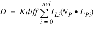
The diffuse component is defined as:
where:
Kdiff is the diffuse reflectance coefficient.
ILi is the intensity of light source
i. NP is the unit surface normal at point
P. LPi is the unit vector from point
P to the location of the point light source
Li. By default, nvl is the total number of lights. If the Shadows keyword is specified in the call to RENDER, then nvl is the number of visible light sources (possibly via transmission through objects) at point P.
Transmission Component
The transmission component is simply the light which has passed through the object at a particular point. For example, the color of a point on a glass ball is a combination of both the light striking the surface and the light which passes through it from the opposite side of the point. RENDER currently assumes that the refractive indices of all objects are the same.
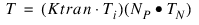
The transmission component is defined as:
where:
Ktran is the specular transmission coefficient.
Ti is the intensity of the light that is transmitted from other objects, assuming that all objects have a refractive index of 1 (air).
NP is the unit surface normal at point
P. TN is the calculated specular transmission microfacet normal from the direction of transmission.
Ambient Component
The ambient component of the resulting shaded color is completely independent of the position of objects and light sources. It is typically used alone (i.e., Kdiff and Ktran are 0) for flat shading and for rendering voxel values as intensities that correspond directly to their actual byte values.
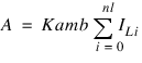
The ambient component is defined as:
where:
Kamb is the ambient coefficient.
nl is the total number of light sources.
ILi is the intensity of light source
i.
Defining Object Material Properties
The following keywords can be used with each RENDER object:
Color—The color (intensity) coefficient of the object.
Kamb—The ambient coefficient (flat shaded).
Kdiff—The diffuse reflectance coefficient.
Ktran—The specular transmission coefficient.
Objects may have up to 256 material properties each; thus, an array of 256 double-precision floating-point values can be assigned to each keyword.
The defaults for these properties vary from object to object:
For CONE, CYLINDER, SPHERE, and MESH,
Color and
Kdiff are all 1, while
Kamb and Ktran are all 0. (This corresponds to
Color(0:255)=1.0 and
Ktran(0:255)=0.0 in PV‑WAVE notation.)
For VOLUME,
Color are all 1,
Kdiff and
Ktran are all 0, and
Kamb is an array of 256 linearly increasing values from 0 to 1.
CONE, CYLINDER, and SPHERE also support a Decal keyword that allows mapping of a byte image onto the surface of the object. The values in the image correspond to an index into the arrays of material properties defined above; thus, different regions on an object can have different properties.
For polygonal meshes, in addition to specifying a list of polygons, you can also specify a 1D array of bytes, one element for each polygon. This array is an index into the arrays of material properties defined above. This allows you to then use the Materials keyword to specify different properties for different polygons.
The actual value in the voxel array of bytes defining a VOLUME is used as an index into the arrays of material properties defined with the Materials keyword; thus, a voxel data set can be considered to be made up of as many as 256 voxel types.
note | For best results, be sure that each Color(Kamb+Kdiff+Ktran) setting is in the range [0...1]. Otherwise, you must use the Scale keyword in the call to RENDER. |
Decals
A decal is a 2D array (image) of bytes whose elements correspond to indices into the arrays of material properties. You can use the Decal keyword with the quadric objects.
For example, if a given point on an object is mapped to coordinates
(u,v) in the decal image, then the material properties used at that point for shading would be
Color(Decal(u,v)),
Kamb(Decal(u,v)),
Kdiff(Decal(u,v)), and
Ktran(Decal(u,v)). An example of applying a decal to a sphere is shown in
"Example 4: Quadric Animation".
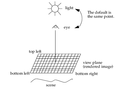
Setting Object and View Transformations
The view that is automatically generated by RENDER is depicted in
Default View for RENDER. (You can retrieve this view with the
Info keyword; for details, see the PV‑WAVE
Reference.)
You can use the View keyword with RENDER to specify a different view. This is especially useful for zooming in or for animations, since changes in scale can result if you use the default view in animations.
You can also use the Transform keyword with any object passed into RENDER. This keyword allows individual objects to be transformed (e.g., rotated, scaled, and positioned) separately from other objects in the scene. Transform contains the local transformation matrix whose default is the identity matrix:
Typically, you would build the transformation matrix by first using the
T3D procedure and then using the system variable transformation matrix
!P.T. Examples of using this method of matrix construction are shown throughout the
"RENDER Examples".
For more information, see the section
"Geometric Transformations".
Invoking RENDER
RENDER is the function that generates the image from the objects you have specified. The general format is:
result = RENDER(object1, ..., objectn)
where objecti is any number of objects previously-defined with the RENDER object functions.
RENDER returns a byte image of size X-by-Y, where X and Y each default to 256 unless overridden by the keywords X and Y. The returned image can then be displayed using either the TV or TVSCL procedure.
As illustrated in
Figure 7-4: Default View for RENDER on page 189, RENDER automatically generates a default view. However, you may choose to use the
View or
Transform keywords to alter this default view.
Unless otherwise specified, a single-point light source is defined to coincide with the observer’s viewpoint. The Lights keyword can be used to pass in an array of locations and intensities of point light sources.
For details on using the other RENDER keywords—Sample, Scale, Shadow, X, Y, and Info—see the description of this function in the PV‑WAVE Reference.
RENDER Examples
The following examples were designed to show the capabilities of RENDER, rather than to depict typical applications. You can find most of the examples in this section in:
(UNIX) <wavedir>/demo/render
(WIN) <wavedir>\demo\render
The data and image files used are in:
(UNIX) <wavedir>/data
(WIN) <wavedir>\data
Where <wavedir> is the main PV-WAVE directory.
Example 1: Polygonal Mesh (Diffusely-shaded Polygons)
This example constructs a polygonal mesh (iso-surface) of diffusely-shaded polygons. The default light source is at the eye-point.
Program Listing
PRO cube1
verts = [[-1.0,-1.0,1.0], [-1.0,1.0,1.0], $
[1.0,1.0,1.0],[1.0,-1.0,1.0], [-1.0,-1.0,-1.0], $
[-1.0,1.0,-1.0], [1.0,1.0,-1.0], [1.0,-1.0,-1.0]]
polys=[4,0,1,2,3, 4,4,5,1,0, 4,2,1,5,6, 4,2,6,7,3, $
4,0,3,7,4, 4,7,6,5,4]
m = MESH(verts, polys)
T3D, /Reset, Rotate = [15.0, 30.0, 45.0]
i = RENDER(m, x = 512, y = 512, Transform = !P.T)
TV, i
END
Example 2: Polygonal Mesh (Flat-shaded Polygons)
This example constructs a polygonal mesh of flat-shaded polygons. Each polygon face has a different intensity, independent of the light source or the eye-point (which are the same here.)
Program Listing
PRO cube2
verts = [[-1.0,-1.0,1.0], [-1.0,1.0,1.0], [1.0,1.0,1.0],$
[1.0,-1.0,1.0], [-1.0,-1.0,-1.0], [-1.0,1.0,-1.0],$
[1.0,1.0,-1.0], [1.0,-1.0,-1.0]]
polys = [4,0,1,2,3, 4,4,5,1,0, 4,2,1,5,6, 4,2,6,7,3, $
4,0,3,7,4, 4,7,6,5,4]
amb = FLTARR(256)
amb(0:5) = [.5, .3, .7, .9, .4, .1]
m = MESH(verts, polys, Materials = [0,1,2,3,4,5], $
Kdiff = FLTARR(256), Kamb = amb)
T3D, /Reset, Rotate = [15.0,30.0,45.0]
i = RENDER(m, x = 512, y = 512, Transform = !P.T)
TV, i
END
Example 3: Polygonal Mesh (Many Polygons)
This example is a realistic application of polygonal meshes. It generates 52,500 polygons (approximately 98,000 triangles) as an iso-surface using the SHADE_VOLUME procedure. The polygons are then rendered.
The resulting image, shown in
Ray-Traced Iso-Surface, is saved to a file and is displayed using
show_iso_head.pro.
Note, however, that it is not necessary to convert to a polygonal representation prior to rendering volumes; this is shown in Examples 5 through 8.
Program Listing
PRO gen_iso_head
; Volume data dimensions
volx = 115 & voly = 75 & volz = 105
; The neighborhood size of the average filter.
band = 5
dat = BYTARR(volx, voly, volz)
OPENR, 1, !Data_Dir + ’man_head.dat’
READU, 1, dat
CLOSE, 1
; Apply band ^ 3 average filter.
head = BYTARR(volx + 2 * band, voly + 2 * band, volz + 2 * band)
head(band:band + volx - 1, band:band + voly - 1, $
band:band + volz - 1) = dat
head = SMOOTH(head, band)
SHADE_VOLUME, head, 18, vertex_list, polygon_list, /Low
; Generate iso-surface.
m = MESH(vertex_list, polygon_list)
T3D, /Reset, Rotate = [60.0,0.0,-60.0]
im = RENDER(m, x = 512, y = 512, Transform = !P.T)
TVSCL, im
OPENW, 1, ’iso_head.img’
WRITEU, 1, im
CLOSE, 1
END
Program Listing
PRO show_iso_head
im = BYTARR(512, 512)
OPENR, 1, !Data_Dir + ’iso_head.img’
READU, 1, im
CLOSE, 1
TVSCL, im
END
Example 4: Quadric Animation
This example “constructs” a movie of an orbit around a sphere which has ocean temperature mapped on as a decal and a color lookup table applied from PV‑WAVE after generation of the movie.
If you wanted to add the boundaries of countries, you could do so by drawing them directly into the decal prior to calling SPHERE.
Note that the movie is saved to a file and is displayed using show_anim.pro.
Program Listing
PRO gen_anim
; Load the decal to apply.
decal = BYTARR(720, 360)
OPENR, 1, !Data_Dir + ’world_map.dat’
READU, 1, decal
CLOSE, 1
; Set shading to correspond directly to image values.
dif = FLTARR(256)
amb = FINDGEN(256)/255.
T3D, /Reset, Rotate = [-90.0, 90.0, 0.0]
c = SPHERE(Decal = decal, Kamb = amb, Kdiff = dif, $
Transform = !P.T)
mve = BYTARR(256, 256, 72)
FOR i = 0, 71 DO BEGIN
T3D, /Reset, Rotate = [-20.0, i*5.0, 0.0]
; Create an animation by orbiting view around the sphere.
mve(*, *, i) = RENDER(c, x = 256, y = 256, Transform = !P.T)
ENDFOR
OPENW, 1, !Data_Dir + ’world_anim.img’
WRITEU, 1, mve
CLOSE, 1
END
Program Listing
FUNC show_anim
Window, 0, XSize = 256, YSize = 256, Colors = 128,$
XPos = 300,YPos = 50
red = FLTARR(256)
grn = FLTARR(256)
blu1 = FLTARR(256)
blu2 = FLTARR(256)
; Create a color lookup table.
FOR i=0, 100 DO BEGIN
fi = FLOAT(i)
red(i) = (-((ABS(fi - 100.0)^2.00)))
grn(i) = (-((ABS(fi - 50.0)^1.50)))
blu1(i) = (-((ABS(fi - 25.0)^1.00)))
blu2(i) = (-((ABS(fi - 100.0)^0.50)))
ENDFOR
red = BYTSCL(red)
grn = BYTSCL(grn)
blu = BYTSCL(blu1) > BYTSCL(blu2)
TVLCT, red, grn, blu, 0
white = 127 & TVLCT, 255, 255, 255, white
light_yellow = 126 & TVLCT, 255, 255, 127, light_yellow
light_purple = 125 & TVLCT, 255, 127, 255, light_purple
light_cyan = 124 & TVLCT, 127, 255, 255, light_cyan
yellow = 123 & TVLCT, 255, 255, 000, yellow
purple = 122 & TVLCT, 255, 000, 255, purple
cyan = 121 & TVLCT, 000, 255, 255, cyan
light_red = 120 & TVLCT, 255, 127, 127, light_red
light_green = 119 & TVLCT, 127, 255, 127, light_green
light_blue = 118 & TVLCT, 127, 127, 255, light_blue
greenish_red = 117 & TVLCT, 255, 127, 000, greenish_red
redish_green = 116 & TVLCT, 127, 255, 000, redish_green
redish_blue = 115 & TVLCT, 127, 000, 255, redish_blue
bluish_red = 114 & TVLCT, 255, 000, 127, bluish_red
bluish_green = 113 & TVLCT, 000, 255, 127, bluish_green
greenish_blue = 112 & TVLCT, 000, 127, 255, greenish_blue
red = 111 & TVLCT, 255, 000, 000, red
green = 110 & TVLCT, 000, 255, 000, green
blue = 109 & TVLCT, 000, 000, 255, blue
gray = 108 & TVLCT, 127, 127, 127, gray
dark_yellow = 107 & TVLCT, 127, 127, 000, dark_yellow
dark_purple = 106 & TVLCT, 127, 000, 127, dark_purple
dark_cyan = 105 & TVLCT, 000, 127, 127, dark_cyan
dark_red = 104 & TVLCT, 127, 000, 000, dark_red
dark_green = 103 & TVLCT, 000, 127, 000, dark_green
dark_blue = 102 & TVLCT, 000, 000, 127, dark_blue
black1 = 101 & TVLCT, 000, 000, 000, black1
black = 000 & TVLCT, 000, 000, 000, black
EMPTY
; Load the previously generated animation.
frames = BYTARR(256, 256, 72)
OPENR, 1, !Data_Dir + ’world_anim.img’
READU, 1, frames
CLOSE, 1
; Display the animation.
MOVIE, frames, Order=0
RETURN, frames
END
Example 5: Slicing a Volume
This example renders selected slices from a large amount of volume data. The resulting image, shown in
Slices Rendered from a Large Volume, is saved to a file and displayed using
show_slic_head.
Program Listing
PRO gen_slic_head
width = 125 & height = 85 & depth = 115
; Use the procedure load_seg_head.pro to load the byte voxel
; data, set all data outside the head to zero, return the
; “segmented head” as HEAD, and return the thresholded surface
; of the head as SKULL.
load_seg_head, head, skull
vox = BYTARR(width, height, depth)
; Generate the slices of segmented data we wish to view.
FOR i=0,depth-2,20 DO BEGIN
vox(*,*,i) = head(*,*,i)
vox(*,*,i+1) = head(*,*,i+1)
ENDFOR
v = VOLUME(vox)
T3D, /Reset, Rotate = [60.0,0.0,-45.0]
im = RENDER(v, x = 512, y = 512, Transform = !P.T, /Scale)
TVSCL, im
OPENW, 1, !Data_Dir + 'sliced_head.img'
WRITEU, 1, im
CLOSE, 1
END
Program Listing
PRO show_slic_head
im = BYTARR(512, 512)
OPENR, 1, !Data_Dir + 'sliced_head.img'
READU, 1, im
CLOSE, 1
TVSCL, im
END
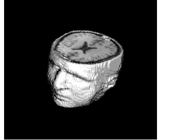
Example 6: Rendering an Iso-Surface with Voxel Values
This example renders a diffuse iso-surface using actual voxel values. The results, shown in
Cutaway Human Head, are saved to a file and displayed using
show_flat_head.
Program Listing
PRO gen_flat_head
width = 125 & height = 85 & depth = 115
; Use the procedure load_seg_head.pro to load the byte
; voxel data, set all data outside the head to zero,
; return the ’segmented head’ as HEAD, and return the
; thresholded surface of the head as SKULL.
load_seg_head, head, skull
overlap = skull * head
overlap(where(overlap GT 0)) = 1
; Remove portion of head that overlaps with skull.
head = head * (BYTE(1) - overlap)
vox = BYTARR(width, height, depth)
; Generate the slices of smoothed data we wish to view.
FOR i=0,76 DO vox(*,*,i) = $
head(*, *, i) + (skull(*, *, i)*BYTE(255))
; Voxel value 255 is special, representing the skull surface.
diff = FLTARR(256) & diff(255) = 0.6
amb = FINDGEN(256)/255.0 & amb(255) = 0.0
v = VOLUME(vox, Kdiff = diff, Kamb = amb)
T3D, /Reset, Rotate = [60.0, 0.0, -45.0]
im = RENDER(v, x = 512, y = 512, Transform = !P.T, /Scale)
TVSCL, im
OPENW, 1, !Data_Dir + ’flat_head.img’
WRITEU, 1, im
CLOSE, 1
END
Program Listing
PRO show_flat_head
im = BYTARR(512,512)
OPENR, 1, !Data_Dir + ’flat_head.img’
READU, 1, im
CLOSE, 1
TVSCL, im
END
Example 7: Diffuse and Partially Transparent Iso-Surfaces
This example renders a diffuse iso-surface and a partially transparent iso-surface. The results, shown in
Figure 7-8: Head with Transparent Surface on page 201, are saved to a file and displayed using
show_tran_head.
Program Listing
PRO gen_tran_head
width = 125 & height = 85 & depth = 115
; Use the procedure load_seg_head.pro to load the byte
; voxel data, set all data outside the head to zero,
; return the ’segmented head’ as HEAD, and return the
; thresholded surface of the head as SKULL.
; See the file load_seg_head.pro (in the wave/demo/render
; directory).
load_seg_head, head, skull
; Generate a mask plane that will split head in half,
; allowing half to be diffuse and rest to be transparent.
mask = BYTARR(width, height, depth)
mask(*, height/2:*, *) = 1
; Half surface = 255, other half = 254
skull * (BYTE(1) - mask) * BYTE(254)
; Remove portion of head that overlaps with skull.
overlap = skull * head
overlap(WHERE(overlap GT 0)) = 1
head = head * (BYTE(1) - overlap)
; Voxel value 255 is special, corresponding to surface of
; half head. Value 254 corresponds to surface of other
; half. Remaining values are actual unsmoothed head data
; and are not used for this example (i.e., they are completely
; transparent).
vox = shell + head
diff = FLTARR(256) & diff(255) = 1.0 & diff(254) = 0.05
tran = FLTARR(256) & tran(*) = 1.0 & tran(255) = 0.0
tran(254) = 0.95
v = VOLUME(vox, Ktran = tran, Kamb = FLTARR(256), $
Kdiff = diff)
T3D, /Reset, Rotate = [60.0, 0.0, -45.0]
im = RENDER(v, x = 512, y = 512, Transform = !P.T)
TVSCL, im
OPENW, 1, !Data_Dir + ’trans_head.img’
WRITEU, 1, im
CLOSE, 1
END
Program Listing
PRO show_tran_head
im = BYTARR(512, 512)
OPENR, 1, !Data_Dir + ’trans_head.img’
READU, 1, im
CLOSE, 1
TVSCL, im
END
Example 8: Rendering Iso-Surfaces with Transformation Matrices
This example renders two diffuse iso-surfaces as well as actual voxel values. The results, shown in
Two Volumes in One Image, are saved to a file and displayed using
show_core_head.
Program Listing
PRO gen_core_head
width = 125 & height = 85 & depth = 115
; Use the procedure load_seg_head.pro to load the byte
; voxel data, set all data outside the head to zero,
; return the ’segmented head’ as HEAD, and return the
; thresholded surface of the head as SKULL.
load_seg_head, head, skull
overlap = skull * head
overlap(WHERE(overlap GT 0)) = 1
; Remove portion of head that overlaps with skull.
head = head * (BYTE(1) - overlap)
vox = head + (skull * BYTE(255))
; Create a circle (used for CYLINDER) mask plane.
circle = BYTARR(width, height)
radius2 = 16 * 16
FOR x=0, width-1 DO BEGIN
dx = x - width / 2
dx = dx * dx
FOR y=0, height-1 DO BEGIN
dy = y - height / 2
dy = dy * dy
IF ((dx + dy) LE radius2) THEN BEGIN
circle(x, y) = 1
ENDIF
ENDFOR
ENDFOR
; Mask out the core sample and "subtract" out from slices.
core = BYTARR(width, height, depth)
FOR z=0, depth-1 DO BEGIN
core(*, *, z) = vox(*, *, z) * circle
vox(*, *, z) = vox(*, *, z) - core(*, *, z)
ENDFOR
; Voxel value 255 is special, representing the skull surface.
diff = FLTARR(256) & diff(255) = 0.6
amb = FINDGEN(256)/255.0 & amb(255) = 0.0
; Surface and interior of skull.
v0 = VOLUME(vox, Kdiff = diff, Kamb = amb)
T3D, /Reset, Translate=[0.0, 0.0, 1.0]
; Core sample.
v1 = VOLUME(core, Transform = !P.T, Kdiff = diff, Kamb = amb)
T3D, /Reset, Rotate = [60.0, 0.0, -45.0]
im = RENDER(v0, v1, x = 512, y = 512, Transform = !P.T, /Scale)
TVSCL, im
OPENW, 1, !Data_Dir + ’core_head.img’
WRITEU, 1, im
CLOSE, 1
END
Program Listing
PRO show_core_head
im = BYTARR(512, 512)
OPENR, 1, !Data_Dir + ’core_head.img’
READU, 1, im
CLOSE, 1
TVSCL, im
END
Version 2017.1
Copyright © 2019, Rogue Wave Software, Inc. All Rights Reserved.