Drawing Three-dimensional Graphics
Points in XYZ space are expressed by vectors of homogeneous coordinates. These vectors are translated, rotated, scaled, and projected onto the two-dimensional drawing surface by multiplying them by transformation matrices. The geometrical transformations used by PV‑WAVE, and many other graphics packages, are taken from Chapters 7 and 8 of Fundamentals of Interactive Computer Graphics by J. D. Foley and A. Van Dam (Addison Wesley Publishing Co., 1982). Consult this book for a detailed description of homogeneous coordinates and transformation matrices, as this section presents only an overview.
Overview of Homogeneous Coordinates
A point in homogeneous coordinates is represented as a four-element column vector of three coordinates and a scale factor w ≠ 0:
P(wx, wy, wz, w) ≡ P(x / w, y / w, z / w, 1) ≡ (x, y, z)
One advantage of this approach is that translation, which normally must be expressed as an addition, may be represented as a matrix multiplication. Another advantage is that homogeneous coordinate representations simplify perspective transformations.
PV‑WAVE Coordinate System
The coordinate system is right-handed so that when looking from a positive axis to the origin a positive rotation is counterclockwise. As usual, the x-axis runs across the display, the y-axis is vertical, and the positive Z axis extends out from the display to the viewer. A 90 degree positive rotation about the Z axis transforms the X axis to the Y axis.
Overview of Transformation Matrices
For most applications, it is not necessary to create, manipulate, or to even understand transformation matrices. The T3D procedure, explained below, implements most of the common transformations.
Transformation matrices, which post-multiply a point vector to produce a new point vector, must be (4,4). A series of transformation matrices may be concatenated into a single matrix by multiplication. If A1, A2, and A3 are transformation matrices to be applied in order, and the matrix A is the product of the three matrices:
((P · A1) · A2) · A3 ≡ P · ((A1 · A2) · A3) = P · A
A = (A1 · A2) · A3
PV‑WAVE stores the concatenated transformation matrix in the system variable field !P.T.
Each of the operations of translation, scaling, rotation, and shearing may be represented by a transformation matrix.
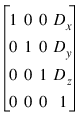
Translating Data
The transformation matrix to translate a point by (Dx, Dy, Dz) is:
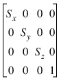
Scaling Data
Scaling by factors of Sx, Sy, and Sz, about the x-, y- and z-axes respectively is represented by the matrix:
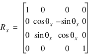
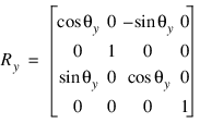
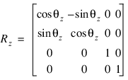
Rotating Data
Rotation about the x-, y-, and z-axes is represented respectively by the three matrices:
Clipping 3D Plots
Clipping consists of defining a specific region in a plot where existing data is plotted, and outside of which no data are shown. The general concept of clipping and the use of clipping for two-dimensional plots is discussed in
Displaying 2D Data. Keywords provided with the PV‑WAVE graphics commands let you specify how clipping is done.
Notes on the Keywords and System Variables for 3D Clipping
When you call CONTOUR or SURFACE, the value of !P.Clip is set to a default value. This value depends on the current device. Setting the Clip keyword has no effect on !P.Clip.
Graphics keywords for controlling clipping are discussed in detail in
Displaying 2D Data of this manual, and are summarized in
"Notes on the Keywords and System Variables".
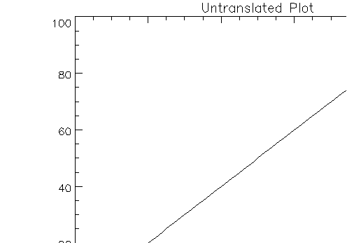
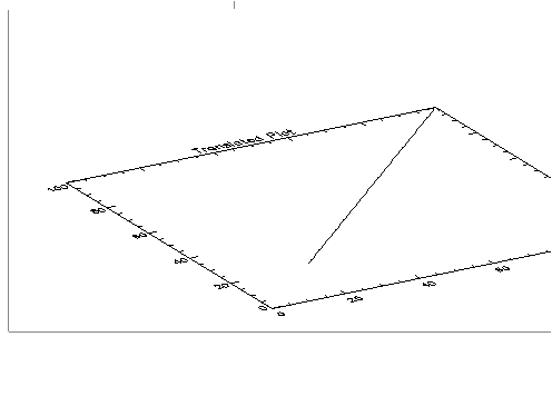
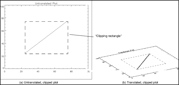
If you use clipping in a three-dimensional plot and you rotate the plot in three dimensions, you may notice some unusual clipping behavior. For instance, some part of your plot may be clipped in 3D when it was not clipped in 2D, as shown in the following example. Note the clipping “problem” encountered when these two plots are compared:
; Produce the first plot—a simple line plot.
PLOT, INDGEN(100)
SURFR
; Produce the second plot—a simple line plot translated to 3D.
PLOT, INDGEN(100), /T3D
Figure 5-12: Translating a Line Plot on page 105 shows two pictures. The first picture shows a simple line plot. In the second, the same plot is shown translated in 3D. The translated plot appears to be missing some data near the origin.
The key to clipping in three dimensions is to remember that the !P.Clip system variable defines a default clipping rectangle that a) is always in device coordinates and b) cannot be translated to 3D coordinates.
Translated, Clipped Line Plot shows clearly why the rotated graphic was clipped by the default clipping rectangle.
; Show the coordinates of the default clipping rectangle defined
; by !P.Clip.
PRINT, !P.Clip
; PV-WAVE prints: 90 72 613 476 0 6
In this figure, a dashed line was drawn connecting the coordinates defining the corners of the default clipping rectangle. The coordinates of these corners were taken directly from !P.Clip. The dashed lines show clearly the boundary of this clipping rectangle. Part of the data (near the origin) falls outside this rectangle, and that is why it is clipped.
The data in a translated graphic can be clipped by the default clipping rectangle, which cannot be rotated. This unwanted clipping behavior can be avoided by adding the /NoClip keyword to the command that produces the rotated graphic.
You can avoid unwanted clipping of translated plots by adding the
NoClip keyword to the graphics command, as shown in
Translated Line Plot with NoClip Specified.
PLOT, INDGEN(100), /T3D, /NoClip
The same translated plot is produced, but this time the data near the origin is not clipped.
The clipping rectangle defined by the
Clip keyword is translated along with the plot for which it is defined as shown in
Translated Line Plot with Clip Specified. You can use
Clip to modify a plot, and the clipping is preserved when you translate or rotate the plot in 3D.
PLOT, INDGEN(100), Clip=[25,25,75,75]
SURFR
PLOT, INDGEN(100), Clip=[25,25,75,75], /T3D
Using the T3D Procedure to Transform Data
The T3D procedure creates and accumulates transformation matrices, storing them in the system variable field !P.T. It can be used to create a transformation matrix composed of any combination of translation, scaling, rotation, perspective projection, oblique projection, and axis exchange.
Keywords that affect transformations are applied in the order of their description below:
 Reset
Reset—Resets the transformation matrix to the identity matrix to begin a new accumulation of transformations. If this keyword is not present, the current transformation matrix !P.T is post-multiplied by the new transformation. The final transformation matrix is always stored back in !P.T.
Translate—Translates by the three-element vector [
Tx, Ty, Tz]. Scale—Scales by factor [
Sz, Sy, Sz].
Rotate—Rotates about each axis by the amount [
θx,
θy,
θz], in degrees.
Perspective—A scalar (p) indicating the
z distance of the center of the projection in the negative direction. Objects are projected into the XY plane, at Z = 0, and the “eye” is at point (0, 0, –
p).
Oblique—A two-element vector, [
d,
α], specifying the parameters for an oblique projection. Points are projected onto the XY plane at
z = 0 as follows:
x' = x + z(d cos α)
y' = y + z(d sin α)
An oblique projection is a parallel projection in which the normal to the projection plane is the z-axis, and the unit vector (0, 0, 1) is projected to (d cos α, d sin α).
XYexch—If set, exchanges the
x- and
y-axes.
XZexch—If set, exchanges the
x- and
z-axes.
YZexch—If set, exchanges the
y- and
z-axes.
An Example of Transformations Created by SURFACE
The SURFACE procedure creates a transformation matrix from its keyword parameters AX and AZ as follows:
It translates the data so that the center of the normalized cube is moved to the origin.
It rotates –90 degrees about the
x-axis to make the +
z-axis of the data the +
y-axis of the display. The +
y data axis extends from the front of the display to the rear.
It rotates about the
y-axis
AZ degrees. This rotates the result counterclockwise as seen from above the page.
It rotates about the
x-axis
AX degrees, tilting the data towards the viewer.
It then translates back to the origin and scales the data so that the data are still contained within the normal coordinate unit cube after transformation.
These transformations can be created using T3D as shown below. The SURFR (SURFace Rotate) procedure mimics the transformation matrix created by SURFACE using this method.
; Translate to move center of cube to origin.
T3D, /Reset, Translate=[-.5, -.5, -.5]
; Rotate –90 degrees about x-axis, so +z-axis is now +y.
; Then rotate about y-axis AZ degrees.
T3D, Rotate=[-90, az, 0]
; Rotate AX about x-axis.
T3D, Rotate=[ax, 0, 0]
; This procedure scales !P.T so that the unit cube still fits
; within the unit cube after transformation.
SCALE3D
Converting from 3D to 2D Coordinates
To convert from a three-dimensional coordinate to a two-dimensional coordinate, PV‑WAVE follows these steps:
Data coordinates are converted to three-dimensional normalized coordinates. As described in
"Coordinate System Conversion", to convert the X coordinate from data to normalized coordinates:
Nx = X0 + X1Dx
where X1 is !X.S(i). The same process is used to convert the Y and Z coordinates using !Y.S and !Z.S.
The three-dimensional normalized coordinate,
P = (
Nx,
Ny,
Nz), whose homogeneous representation is (
Nx,
Ny,
Nz, 1), is multiplied by the concatenated transformation matrix !P.T:
P' = P · !P.T
N'x = P'x / P'w and N'y = P'y / P'w
This process can be written as a PV‑WAVE function:
; Accept a 3D data coordinate, return a two-element vector
; containing the coordinate transformed to 2D normalized
; coordinates using the current transformation matrix.
FUNCTION CVT_TO_2D, x, y, z
; Make a homogeneous vector of normalized 3D coordinates.
p = [!x.s(0) + !x.s(1) * x, !y.s(0) + !y.s(1) $
* y, !z.s(0) + !z.s(1) * z, 1]
; Transform by !P.T.
p = p # !P.T
; Return the scaled result as a two-element, 2D, XY vector.
RETURN, [ p(0) / p(3), p(1) / p(3) ]
END
Establishing Your Own 3D Coordinate System
Usually, scaling parameters for coordinate conversion are set up by the higher-level plotting procedures. To set up your own 3D coordinate system with a given transformation matrix and X, Y, Z data range, follow these steps:
Establish the scaling from your data coordinates to normalized coordinates—the (0,1) cube. Assuming your data are contained in the range (
Xmin,
Ymin,
Zmin) to (
Xmax,
Ymax,
Zmax), set the data scaling system variables as follows:
!X.S = [ -Xmin, 1 ] / (Xmax - Xmin)
!Y.S = [ -Ymin, 1 ] / (ymax - Ymin)
!Z.S = [ -Zmin, 1 ] / (Zmax - Zmin)
Establish the transformation matrix which determines the view of the unit cube. This can be done by either calling T3D, explained above, or by directly manipulating !P.T yourself. If you wish to simply mimic the rotations provided by the SURFACE procedure, call the SURFR procedure.
Call the SCALE3D procedure to re-scale the projected unit cube back to the (0,1) 2D normalized coordinate square. SCALE3D transforms a unit cube by the current !P.T and uses the extrema of each axis to translate and rescale the result back to the unit square.
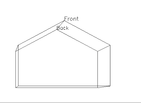
Example of Data Transformations
This example draws four views of a simple house. The procedure HOUSE defines the coordinates of the front and back faces of the house. The data to normal coordinate scaling is set, as shown above, to a volume about 25% larger than that enclosing the house. The PLOTS procedure draws lines describing and connecting the front and back faces. XYOUTS is called to label the front and back faces.
The main program contains four sequences of calls to T3D to establish the coordinate transformation, followed by a call to SCALE3D to center the transformed unit cube in the viewing area, and then by a call to HOUSE.
note | Remember that a valid data coordinate system must be established before calling PLOTS. This coordinate system can be established by a call to PLOT, or by explicitly setting values of the system variables !X, !Y, and !Z. |
Procedure Used to Draw a House
Define a procedure to draw a house.
PRO HOUSE
; The X coordinates of 10 vertices. First 5 are front face,
; second 5 are back face. Range is 0 to 16.
house_x = [0, 16, 16, 8, 0, 0, 16, 16, 8, 0]
; Corresponding y values. Range is 0 to 16.
house_y = [0, 0, 10, 16, 10, 0, 0, 10, 16, 10]
; Z values, from 30 to 54.
house_z = [54, 54, 54, 54, 54, 30, 30, 30, 30, 30]
; Set x data scale to range from –4 to 20.
!X.S = [-(-4), 1.] / (20 - (-4))
; Same for y.
!Y.S = !x.s
; Z range is from 10 to 70.
!Z.S = [-10, 1. ] / (70 - 10)
; Indices of front face.
face = [INDGEN(5), 0]
; Draw front face.
PLOTS, house_x(face), house_y(face), house_z(face), /T3D, $
/Data
; Draw back face.
PLOTS, house_x(face+5), house_y(face+5), house_z(face+5), $
/T3D, /Data
; Connecting lines from front to back.
FOR i=0, 4 DO PLOTS, [house_x(i), $
house_x(i+5)], [house_y(i), $
house_y(i+5)], [house_z(i), $
house_z(i+5)], /T3D, /Data
; Annotate front peak.
XYOUTS, house_x(3), house_y(3), Z=house_z(3), 'Front', $
/T3D, /Data, Size=2
; Annotate back.
XYOUTS, house_x(8), house_y(8), Z=house_z(8), 'Back', /T3d, $
/Data, Size = 2
END
Commands that Perform Transformations on the House
The following commands demonstrate the 3D transfomations shown in
3D Transformations.
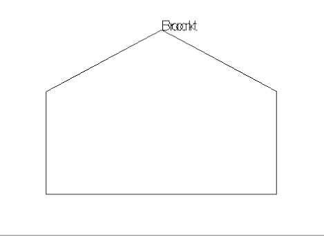
; Set up no rotation, scale, and draw house.
T3D, /Reset & SCALE3D & house
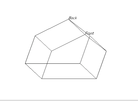
; Straight projection after rotating 30 degrees about x- and
; y-axes.
T3D, /Reset, rot=[30, 30, 0] & SCALE3D & HOUSE
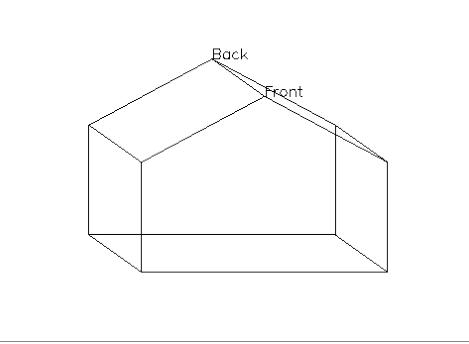
; No rotation, oblique projection, Z factor = 0.5, angle = 45.
T3D, /Reset, rot=[0, 0, 0], oblique = [.5, -45] & SCALE3D & HOUSE
; No rotation, perspective at 4.
T3D, /Reset, rot = [0, 0, 0], perspective = 4 & SCALE3D & HOUSE
From top: No rotation, plain projection; Rotation of 30 degrees about both the x- and y-axes, plain projection; Oblique projection, factor = 0.5, angle = –45; and in the bottom right, 30 degrees rotation with the eye at 50.
Version 2017.1
Copyright © 2019, Rogue Wave Software, Inc. All Rights Reserved.