3D Transformations with 2D Procedures

User Guide > Displaying 3D Data > 3D Transformations with 2D Procedures

The CONTOUR and PLOT procedures output their results using the three-dimensional coordinate transformation contained in !P.T, if the keyword T3d is specified.

note	!P. T must contain a valid transformation matrix prior to using the T3d keyword.

The PLOT procedures output graphs in the XY plane at the normal coordinate z value given by the keyword ZValue. If ZValue is not specified, the plot is drawn at the bottom of the unit cube, at z=0.

CONTOUR draws axes at Z=0, and contours at their Z data value if ZValue is not specified. If ZValue is present, CONTOUR draws both the axes and contours in the XY plane at the given Z value.

Combining CONTOUR and SURFACE Procedures

You can combine the output of SURFACE with the other graphics procedures. The keyword Save causes SURFACE to save the graphic transformation it used in !P.T. Then, when CONTOUR or PLOT are called with the keyword T3d, their output is transformed with the same projection.

For example, Figure 5-17: Combined Contour and Surface Plots on page 118 illustrates SURFACE combined with CONTOUR. In essence, this a combination of Figure 5-2: Improved Contour Plot on page 88 and Figure 5-11: Maroon Bells Surface Plots on page 100. Using the same variables as discussed in "Drawing Contour Plots with CONTOUR" and "Drawing a Surface", this figure was produced with the following statements:

; Make the mesh.

SURFACE, c, x, y, SKIRT=2650, /Save

; Make Contour plot. Specify T3D to align with Surface, at ZVALUE

; of 1.0. Suppress clipping as plot is outside normal plot window.

CONTOUR, b, x, y, /T3d, /Noerase, Title = 'Contour Plot', $
Max_val=5000., Zvalue = 1.0, /Noclip, Levels = 2750. + $
FINDGEN(6)*250

Figure 5-17: Combined Contour and Surface Plots

Even More Complicated Transformations are Possible

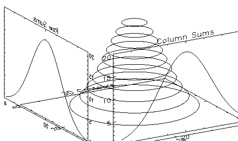
PLOT and CONTOUR with 3D Transformations illustrates the application of three-dimensional transforms to the output of CONTOUR and PLOT. It shows a three-dimensional contour plot with the contours stacked above the axes in the Z direction, the sum of the columns, also a Gaussian, in the XZ plane, and the sum of the rows in the YZ plane.

Figure 5-18: PLOT and CONTOUR with 3D Transformations

The code used to draw Figure 5-18: PLOT and CONTOUR with 3D Transformations on page 118 is:

nx=40

temp = SHIFT(DIST(40), 20, 20)

z = EXP(-(temp/10)^2)

; Define 3D plot window. X = .1 to 1, Y = .1 to 1, 1 and Z = 0 to 1.

pos = [.1, .1, 1, 1, 0, 1]

; Make the stacked contours. Use 10 contour levels.

CONTOUR, z, /T3D, NLEVELS=10, /Noclip, Position = pos, $
Charsize = 2

; Swap y- and z-axes. The original XYZ system is now XZY.

T3D, /Yzexch

; Plot the column sums in front of the contour plot.

PLOT, z # REPLICATE( 1., nx), /Noerase, /Noclip, /T3d, $
Title = 'Column Sums', Position=pos, Charsize=2

; Swap x- and z-axes,original XYZ is now YZX.

T3D, /Xzexch

PLOT, REPLICATE( 1., nx) # z, /Noerase, /T3d, /Noclip, $
Title = 'Row Sums', Position = pos, Charsize = 2

The basic steps are:

First, the SURFR procedure is called to establish the default three-to two-dimensional transformation used by SURFACE, as explained above. The default rotations are 30 degrees about both the x- and z-axes.

Next, a vector, pos, defining the cube containing the plot window is defined with normalized coordinates. The cube extends from 0.1 to 1.0 in the x and y directions, and from 0 to 1 in the Z direction. Each call to CONTOUR and PLOT must explicitly specify this window to align the plots. This is necessary because the default margins around the plot window are different in each direction.

CONTOUR is called to draw the stacked contours with the axes at Z=0. Clipping is disabled to allow drawing outside the default plot window which is only two-dimensional.

The T3D procedure is called to exchange the y- and z-axes. The original XYZ coordinate system is now XZY.

PLOT is called to draw the column sums which appear in front of the contour plot. The expression:

z # REPLICATE(1., nx)

creates a row vector containing the sum of each column in the two-dimensional array z. The Noerase and Noclip keywords are specified to prevent erasure and clipping. This plot appears in the XZ plane because of the previous axis exchange.

T3D is called again to exchange the x- and z-axes. This makes the original XYZ coordinate system, which was converted to XZY, now correspond to YZX.

PLOT is called to produce the row sums in the YZ plane in the same manner as the first plot. The original x-axis is drawn in the Y plane, and the y-axis is in the Z plane. One unavoidable side effect of this method is that the annotation of this plot is backwards. If the plot is transformed so the letters read correctly, the x-axis of the plot would be reversed in relation to the y-axis of the contour plot.

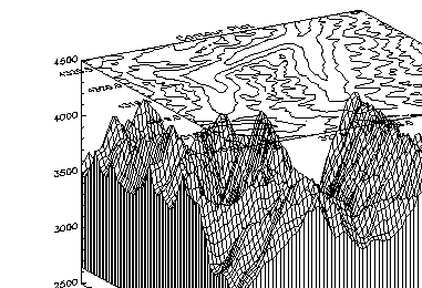
Combining Images with 3D Graphics

Images are combined with 3D graphics, as shown in Combined Image, Surface Mesh, and Contour, using the transformation techniques described in the previous section.

Figure 5-19: Combined Image, Surface Mesh, and Contour

The rectangular image must be transformed so that it fits underneath the mesh drawn by SURFACE. The general approach is as follows:

Use SURFACE to establish the general scaling and geometrical transformation. Draw no data, as the graphics made by SURFACE will be over-written by the transformed image.

For each of the four corners of the image, translate the data coordinate, which is simply the subscript of the corner, into a device coordinate. The data coordinates of the four corners of an (m, n) image are (0,0),
(m – 1, 0), (0, n – 1), and (m – 1, n – 1). Call this data coordinate system
(X, Y). Using a procedure or function similar to CVT_TO_2D, described in "Converting from 3D to 2D Coordinates", convert to device coordinates, which in this discussion are called (U, V).

The image is transformed from the original XY coordinates to a new image in UV coordinates using the POLY_2D function. POLY_2D accepts an input image and the coefficients of a polynomial in UV giving the XY coordinates in the original image. The equations for X and Y are:

X = S0,0 + S0,1U + S1,0V + S1,1UV

Y = T0,0 + T0,1U + T1,0V + T1,1UV

We solve for the four unknown S coefficients using the four equations relating the X corner coordinates to their U coordinates. The T coefficients are similarly found using the Y and V coordinates. This can be done using matrix operators and inversion or, more simply, with the POLYWARP procedure.

The new image is a rectangle which encloses the quadrilateral described by the UV coordinates. Its size is:

(max(U) – min(U) + 1, max(V) – min(V) + 1)

POLY_2D is called to form the new image which is displayed at device coordinate (min(U), min(V)).

SURFACE is called once again to display the mesh surface over the image.

Finally, CONTOUR is called, with ZValue set to 1.0, placing the contour above both the image and the surface.

The SHOW3 procedure performs these operations. Look at the code for the SHOW3 procedure in the Standard Library for details of how images and graphics can be combined.

Version 2017.1